Download UPD Grafico Velocimetro Excel
How to Create a Stunning Speedometer Chart in Excel with Grafico Velocimetro
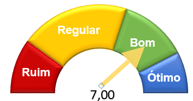
If you want to impress your boss or colleagues with a dynamic and eye-catching data visualization, you might want to try creating a speedometer chart in Excel. A speedometer chart (also known as a gauge chart or a dial chart) is a type of chart that resembles a car’s speedometer and shows how a value compares to a target or a range of values.
In this article, you will learn how to create a speedometer chart in Excel using Grafico Velocimetro, a free and easy tool that you can download from the internet. Grafico Velocimetro is a template that allows you to create speedometer charts in Excel without using any macros or complex formulas. You just need to enter your data and adjust some settings, and you will have a beautiful and professional-looking speedometer chart in minutes.
Step 1: Download Grafico Velocimetro Excel
The first step is to download Grafico Velocimetro Excel from the internet. You can find it on various websites, such as Automate Excel, Hashtag Treinamentos or Excel Total. Just make sure you download the version that matches your Excel language (English, Spanish, Portuguese, etc.).
Once you download the file, you will see that it contains two worksheets: one with instructions and one with the template. You can delete or hide the instructions worksheet if you don’t need it.
Step 2: Enter Your Data
The next step is to enter your data in the template worksheet. You will see that there are four columns: Labels, Levels, Pointer and Total. Here is what each column means:
- Labels: These are the labels that will appear on the speedometer chart. You can use them to indicate the intervals or categories of your data. For example, if you want to show the sales performance of your team, you can use labels such as “Low”, “Medium”, “High” and “Excellent”.
- Levels: These are the values that will determine the size and color of each segment of the speedometer chart. You can use them to set the thresholds or ranges of your data. For example, if you want to show the sales performance of your team, you can use levels such as 0, 24000, 48000, 72000 and 96000.
- Pointer: This is the value that will be displayed by the needle or pointer of the speedometer chart. You can use it to show the current or actual value of your data. For example, if you want to show the sales performance of your team, you can use the pointer to show the total sales of a specific month.
- Total: This is the sum of all the levels. You don’t need to enter this value manually, as it is calculated automatically by the template. You just need to make sure that it is equal to or greater than the pointer value.
For example, if you want to create a speedometer chart that shows the sales performance of your team in January 2023, you can enter your data as follows:
| Labels | Levels | Pointer | Total |
| Low | 0 | 65000 | 96000 |
| Medium | 24000 | ||
| High | 48000 | ||
| Excellent | 72000 | ||
| Total | 96000 |
Step 3: Create the Speedometer Chart
The final step is to create the speedometer chart using Grafico Velocimetro Excel. To do this, you just need to follow these simple steps:
- Format the Doughnut Chart
Now that you have created the doughnut chart, you need to format it to make it look like a speedometer. To do this, you need to follow these steps:
- Right-click on the chart and select Format Chart Area.
- In the Format Chart Area pane, go to the Fill & Line section and select No fill and No line for the chart area.
- Right-click on the doughnut and select Format Data Series.
- In the Format Data Series pane, go to the Series Options section and change the Hole size to 75%.
- In the same pane, go to the Fill & Line section and select No line for the doughnut.
- Select the green segment (Total) and press Delete to remove it from the chart.
- Select each of the remaining segments and change their fill color according to your preference. For example, you can use red for Low, yellow for Medium, green for High and blue for Excellent.
After these steps, your doughnut chart should look something like this:

- Create the Pie Chart
The next step is to create the pie chart that will act as the pointer of the speedometer chart. To do this, you need to follow these steps:
- Select the range G3:G5 and insert a pie chart.
- Delete the legend and the title of the pie chart.
- Right-click on the pie chart and select Select Data.
- In the Select Data Source dialog box, click on Edit under Horizontal (Category) Axis Labels.
- In the Axis Labels dialog box, select the range H3:H5 and click OK.
- In the same dialog box, click on Edit under Legend Entries (Series).
- In the Edit Series dialog box, change the Series name to Pointer and click OK.
- In the same dialog box, click OK again to close it.
- Select each of the segments of the pie chart and change their fill color to white.
- Select only the segment that corresponds to Pointer and change its fill color to black.
- Select any segment of the pie chart and drag it slightly away from the center to create a gap between them.
After these steps, your pie chart should look something like this:

- Align the Two Charts
The final step is to align the two charts (doughnut and pie) to create the speedometer chart. To do this, you need to follow these steps:
- Select both charts by holding down Ctrl and clicking on each one.
- In the ribbon, go to the Format tab under Drawing Tools.
- In the A
- Add the Title and Labels to the Chart
The last step is to add the title and labels to the speedometer chart to make it more informative and attractive. To do this, you need to follow these steps:
- Click on the chart and go to the Design tab under Chart Tools.
- In the Chart Layouts group, click on Add Chart Element and select Chart Title and then Above Chart.
- Type a title for your chart, such as “Sales Performance – January 2023”.
- In the same group, click on Add Chart Element and select Data Labels and then Center.
- Select each of the data labels and format them as you wish. For example, you can change their font size, color, alignment, etc.
- If you want to add labels for the pointer value and the total value, you can use text boxes. To do this, go to the Insert tab and click on Text Box.
- Draw a text box near the pointer and type the pointer value, such as “65,000”. Format the text box as you wish.
- Draw another text box near the total value and type the total value, such as “96,000”. Format the text box as you wish.
After these steps, your speedometer chart should look something like this:

Conclusion
Congratulations! You have successfully created a speedometer chart in Excel using Grafico Velocimetro Excel. You can use this chart to display any kind of data that you want to compare with a target or a range of values. You can also customize the chart according to your preferences and needs.
If you want to download Grafico Velocimetro Excel for free, you can visit one of these websites:
If you want to learn more about how to create amazing charts in Excel, you can check out our other articles on this topic:
We hope you enjoyed this article and learned something new. If you have any questions or feedback, please let us know in the comments section below. Thank you for reading!
- Download Grafico Velocimetro Excel and Boost Your Data Visualization Skills
If you are looking for a way to create stunning and dynamic data visualizations in Excel, you might want to download Grafico Velocimetro Excel, a free and easy tool that allows you to create speedometer charts in Excel without using any macros or complex formulas.
Speedometer charts (also known as gauge charts or dial charts) are a type of chart that resemble a car’s speedometer and show how a value compares to a target or a range of values. They are useful for displaying key performance indicators (KPIs), business results, goals, progress, etc.
In this article, you will learn how to download Grafico Velocimetro Excel from the internet and how to use it to create speedometer charts in Excel with just a few clicks. You will also learn some tips and tricks to customize and enhance your speedometer charts according to your preferences and needs.
How to Download Grafico Velocimetro Excel
The first step is to download Grafico Velocimetro Excel from the internet. You can find it on various websites, such as Automate Excel, Hashtag Treinamentos or Excel Total. Just make sure you download the version that matches your Excel language (English, Spanish, Portuguese, etc.).
Once you download the file, you will see that it contains two worksheets: one with instructions and one with the template. You can delete or hide the instructions worksheet if you don’t need it.
How to Use Grafico Velocimetro Excel
The next step is to use Grafico Velocimetro Excel to create speedometer charts in Excel. To do this, you need to follow these steps:
- Enter your data in the template worksheet. You will see that there are four columns: Labels, Levels, Pointer and Total. Here is what each column means:
- Labels: These are the labels that will appear on the speedometer chart. You can use them to indicate the intervals or categories of your data. For example, if you want to show the sales performance of your team, you can use labels such as “Low”, “Medium”, “High” and “Excellent”.
- Levels: These are the values that will determine the size and color of each segment of the speedometer chart. You can use them to set the thresholds or ranges of your data. For example, if you want to show the sales performance of your team, you can use levels such as 0, 24000, 48000, 72000 and 96000.
- Pointer: This is the value that will be displayed by the needle or pointer of the speedometer chart. You can use it to show the current or actual value of your data. For example, if you want to show the sales performance of your team, you can use the pointer to show the total sales of a specific month.
- Total: This is the sum of all the levels. You don’t need to enter this value manually, as it is calculated automatically by the template. You just need to make sure that it is equal to or greater than the pointer value.
- Create the speedometer chart using Grafico Velocimetro Excel. To do this, you just need to select the range F3:F5 and insert a doughnut chart. Then select the range G3:G5 and insert a pie chart. Then align and format both charts as explained in this article.
- Customize and enhance your speedometer chart according to your preferences and needs. You can change the colors, fonts, sizes, positions, etc. of any element of the chart. You can also add titles, labels, text boxes, etc. to make your chart more informative and attractive.
After these steps, you will have a beautiful and professional-looking speedometer chart in Excel like this:
Conclusion
Grafico Velocimetro Excel is a free and easy tool that allows you to create speedometer charts in Excel without using any macros or complex formulas. You can use it to display any kind of data that you want to compare with a target or a range of values. You can also customize and enhance your speedometer charts according to your preferences and needs.
If you want to download Grafico Velocimetro Excel for free, you can visit one of these websites:
If you want to learn more about how to create amazing charts in Excel, you can check out our other articles on this topic:
We hope you enjoyed this article and learned something new. If you have any questions or feedback, please let us know in the comments section below. Thank you for reading!
https://github.com/1consquaeFcrepbu/voice-changer/blob/master/client/lib/Download%20High%20School%20Musical%202%20Full%20Movie%20and%20Relive%20the%20Magic%20Fun%20Facts%20and%20Behind-the-Scenes%20Stories.md
https://github.com/nasubapso/startbootstrap-landing-page/blob/master/src/assets/Exercice%20Electronique%20De%20Puissance%20Pdf%20Une%20Introduction%20%20llectronique%20de%20Puissance%20avec%20des%20Fiches%20Synthtiques.md
https://github.com/3castmogflorde/questdb/blob/master/.github/Libro%20Yo%20Puedo%20Ben%20Sweetland%20Pdf%2019%20macias%20impact%203.11d%20Discover%20the%20Secrets%20of%20Success%20and%20Happiness.md
https://github.com/9noliOtugi/charts.css/blob/main/src/general/Arcgis%20Engine%20Developer%20Kit%20V.10.1%20Download%20How%20to%20Install%20Authorize%20and%20Use%20It.md
https://github.com/tiosemricon/mocha/blob/master/test/Masterton%20Quimica%20General%20Pdf%20El%20libro%20que%20necesitas%20para%20tu%20curso%20de%20quimica.md
https://github.com/1enimtaubu/shell-operator/blob/main/scripts/Download%20Simcity%20Societies%20Deluxe%20Edition%20Torrent%20and%20Unleash%20Your%20Imagination.md
https://github.com/puncmaXnetsu/eShopOnContainers/blob/dev/img/Descargar%20Lex%20Doctor%209%20Full%20Gratis%20Download%20Aprovecha%20las%20ventajas%20de%20la%20versin%209.1.md
https://github.com/fesranfoeka/DotCi/blob/master/resources/Video%20Marketing%20Blaster%20Pro%20Cracked%20How%20to%20Get%20Unlimited%20Free%20Traffic%20from%20YouTube.md
https://github.com/miviYperda/graphic/blob/main/devdoc/Nelson%20Pediatri%20Turkce%20Indir%20Pdfl%20ocukluk%20a%20Hastalklarnn%20Tm%20Ynleriyle%20Ele%20Alnd%20Esiz%20Bir%20Eser.md
https://github.com/comlatoterc/keeweb/blob/master/desktop/img/Wishes%20Level%20B2.2%20Workbook%20Answers%20Tips%20and%20Tricks%20for%20Mastering%20the%20Language%20Skills.md86646a7979
